Background

Averaging kernels (AKs) quantify the information content of Optimal Estimation (OE) retrieval systems and are key in understanding retrieval uncertainty and error. CLIMCAPS outputs a square, symmetric matrix of AK functions for each retrieval variable at every scene (3 × 3 fields of view) to allow diagnostic evaluation. We explain in detail how CLIMCAPS averaging kernels are calculated in Smith and Barnet (2020), and contrast our method with that originally proposed by Rodgers (2000).

Averaging kernels are used in data inter-comparison studies (Rodgers and Connor, 2003; Maddy and Barnet, 2008; Maddy et al., 2009; Gaudel et al., 2018; Iturbide-Sanchez et al., 2017; Smith and Barnet, 2020) and data assimilation models (Levelt et al., 1998; Clerbaux et al., 2001; Yudin, 2004; Segers et al., 2005; Pierce et al., 2009; Liu et al., 2012). We describe how to convolve external data sources, such as models or radiosondes, to CLIMCAPS profiles in Section 3. 

1. Interpreting CLIMCAPS Averaging Kernels

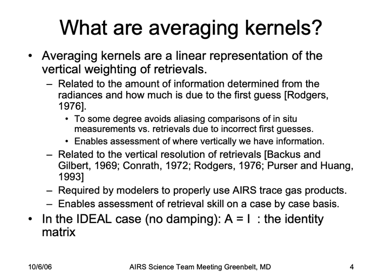
Eric Maddy gave a presentation in 2006 at an AIRS Science Team Meeting specifically focused on AKs.

Maddy et al. 2006: “Application of AIRS V5.0 Averaging Kernels”. AIRS Science Team Meeting, 26-29 Sep 2006, Greenbelt, MD, 

We refer the reader to his presentation because it provides an excellent overview of AKs in general and CLIMCAPS AKs specifically. CLIMCAPS Version 2.0 (V2) is an AIRS Science Team heritage algorithm that is built on the AIRS Version 5.0 method to ensure robust retrievals across the globe and across all seasons, day and night.

Figure 1: An extract from the Maddy et al. 2006 presentation.

Eric Maddy’s seminal paper (Maddy and Barnet, 2008) on averaging kernel application forms the theoretical background to discussions here. Section 3.2 in Nalli et al. (2013) gives a good overview of the Maddy paper with a focus on data validation methods. Iturbide-Sanchez et al. (2017), in turn, discuss how AKs can be interpreted as a metric of vertical resolution.

Our recent paper on CLIMCAPS averaging kernels highlight their value in diagnostic retrieval evaluation. We provide an extract here:

“Averaging kernels are unitless and typically range in value between 0.0 and 1.0, although they can sometimes have negative values where noise exceeds signal. AKs quantify CLIMCAPS observing capability at any given point in time and space because they account for all known sources of scene-specific as well as observing system uncertainty. They characterize a system’s ability to observe a target variable at a specific scene. An alternative interpretation is that they quantify the degree to which the a-priori variable compensates for the lack of observing capability at any specified scene (1.0 – AK). While CLIMCAPS AKs do not measure retrieval accuracy (approximation to the truth), they do characterize retrieval uncertainty and information content. CLIMCAPS retrievals are not in situ measurements of the vertical atmospheric state, but under-determined non-linear inverse measurements with dependence on prior knowledge of the atmospheric state. In scientific analyses and operational applications, it is imperative that sounding observations are correctly interpreted lest their uncertainty is mistaken for measurement. CLIMCAPS AKs characterize and quantify the weighted contribution from the measurement (0.0 + AK) and the a-priori (1.0 – AK) [to the final solution]. An averaging kernel value of zero means that the measurement has no observing capability at that pressure layer and the solution will be the a-priori. An averaging kernel value of unity means the measurement has 100% observing capability and the solution will have no dependence on the a-priori. In practice, however, averaging kernels range in value between these two endpoints such that 0.0 < AK < 1.0.” (Smith and Barnet 2020).

The CLIMCAPS product file contains symmetric AK matrices for every retrieval of temperature (air_temp), water vapor (H₂O_vap), ozone (O₃), methane (CH₄), carbon dioxide (CO₂), carbon monoxide (CO) and nitric acid (HNO₃) irrespective of whether the retrieval passed QC or not. These are reported in the ave_kern/ subgroup with field names suffixed by *_ave_kern. The CLIMCAPS V2 product file does not contain AKs for nitrous oxide (N₂O) and sulphur dioxide (SO₂) because we are unaware of any user applications that require them. This may change in future.

We published different versions of the figures below in Smith and Barnet (2020) with full explanation and discussion. Here, we supplement the discussion in that paper with figures of CLIMCAPS AKs for different seasons and scenes for the sake of a complete representation of CLIMCAPS information content from AIRS/AMSU on Aqua and CrIS/ATMS on JPSS-1.

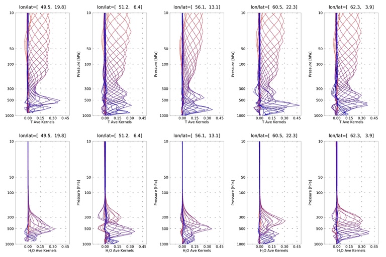
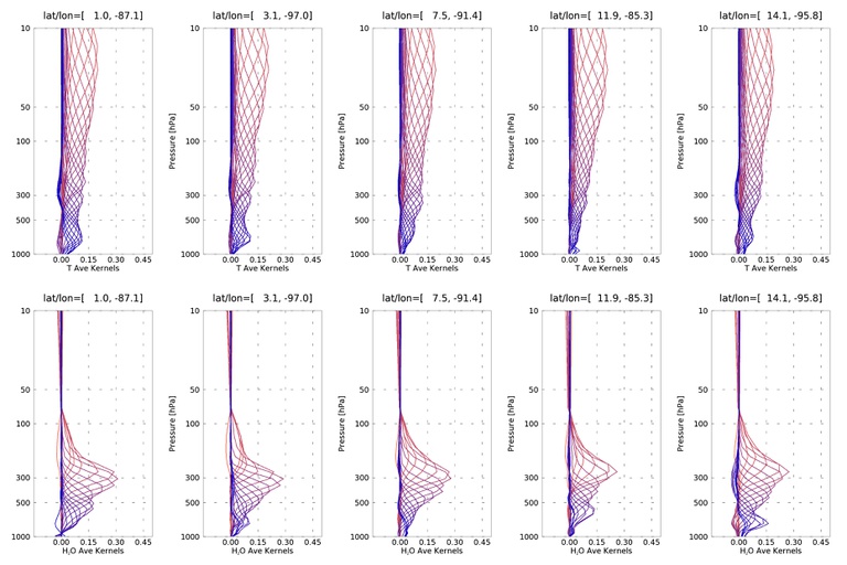
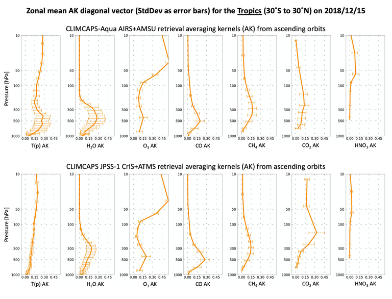
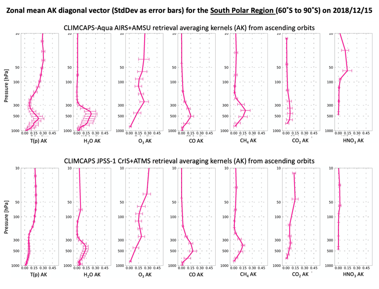
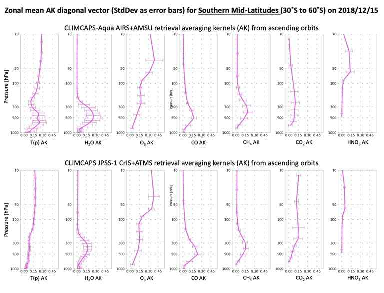
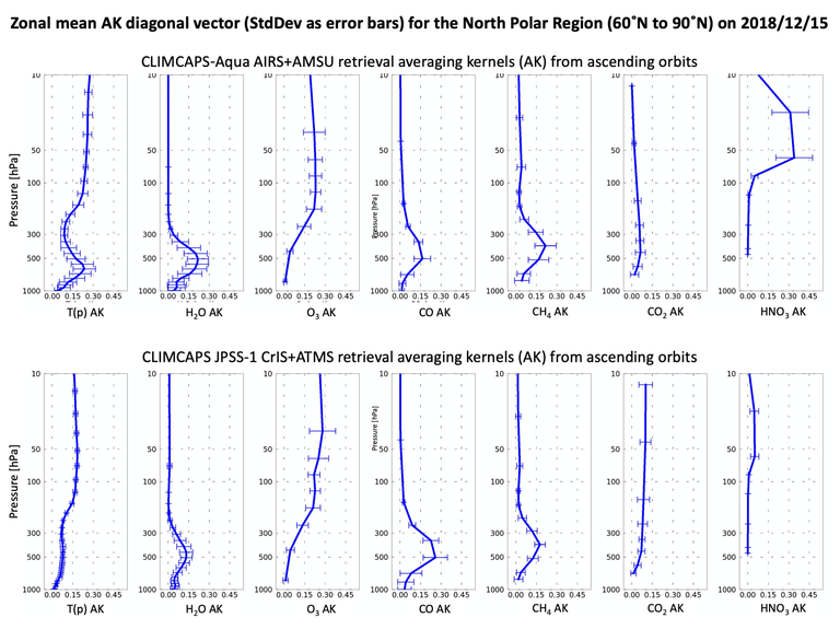
Figure 2 and Figure 3 depict the individual AKs for CLIMCAPS air_temp and H₂O_vap retrievals at specific scenes, while Figure 4, Figure 5, Figure 6 and Figure 7 depict the mean of averaging kernel matrix diagonal vectors for different latitudinal zones on 1 July 2018. The error bars in these figures represent the standard deviation of the diagonal vectors across the latitude zone.

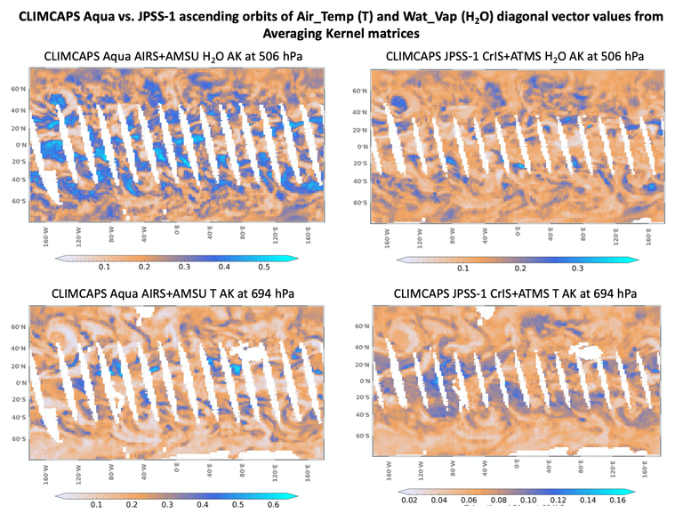
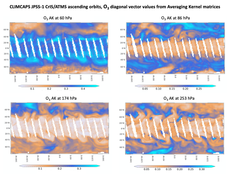
In Figure 8 and Figure 9 we plot the AK diagonal vectors at ~500 hPa for CLIMCAPS H₂O_vap and ~700 hPa for CLIMCAPS air_temp at every retrieval scene to give a global view of information content variability from ascending orbits of CLIMCAPS-Aqua and CLIMCAPS-JPSS1 on 15 December 2018.

We did not apply any quality control filtering to the AK profiles or maps because AKs are not dependent on whether a retrieval succeeds or fails. Instead, averaging kernels depict the potential CLIMCAPS has for retrieving a target variable at each scene. Scenes with much lower (higher) AK values can be interpreted as CLIMCAPS having low (high) information content, and the retrievals probably failed (succeeded).

Figure 2: Scene-dependence of CLIMCAPS-Aqua averaging kernels for coincident (top row) temperature (air_temp) and (bottom row) water vapor (H₂O_vap) retrievals at five scenes (left to right) on 1 July 2018 from Granule 60 with 13h30 local overpass time. The latitude/longitude coordinates are listed at the top of each figure. Averaging kernels quantify and characterize the signal-to-noise ratio of an observing system and are affected by the scene-dependent effects (e.g., temperature lapse rate, amount of gas molecules, surface emissivity and cloud uncertainty) as much as the measurement characteristics (e.g., spectral resolution, instrument calibration and noise). CLIMCAPS retrieves air_temp and H₂O_vap sequentially each with a unique subset of channels, which means that the variation in these averaging kernels are independent of each other.

Figure 3: Same as Figure 2 but for CLIMCAPS-JPSS1 averaging kernels from Granule 97 on 1 July 2018 and 13h30 local overpass time.

Figure 4: The mean (solid line) and standard deviation (error bars) of averaging kernel matrix diagonal vectors in the tropics (30°S to 30°N) on 1 July 2018 and from (top) CLIMCAPS-Aqua and (bottom) CLIMCAPS-JPSS1, both ascending orbits. The error bars indicate the degree to which the averaging kernel diagonal vectors vary spatially across the latitudinal zonal. CLIMCAPS AKs within the northern mid-latitude zone was published and discussed in (Smith and Barnet 2020).

Figure 5: Same as Figure 4 but for southern polar zone (90°S to 60°S). CLIMCAPS AKs within the northern mid-latitude zone was published and discussed in (Smith and Barnet 2020).

Figure 6: Same as Figure 4 but for southern mid-latitude zone (60°S to 30°S). CLIMCAPS AKs within the northern mid-latitude zone was published and discussed in (Smith and Barnet 2020).

Figure 7: Same as Figure 4 but for northern polar zone (60°N to 90°N). CLIMCAPS AKs within the northern mid-latitude zone was published and discussed in (Smith and Barnet 2020).

Figure 8: Spatial variation of CLIMCAPS information content for different retrieval variables and different space-based instruments from their ascending orbits (13h30 local overpass time) on 15 December 2018. (Top row) A global view of CLIMCAPS averaging kernel values at ~500 hPa for H₂O vapor retrievals from (top left) AIRS/AMSU on Aqua, and (top right) CrIS/ATMS on JPSS-1. (Bottom row) A global view of CLIMCAPS averaging kernel values at ~700 hPa for temperature retrievals from (bottom left) AIRS/AMSU on Aqua, and (bottom right) CrIS/ATMS on JPSS-1.

The spatial patterns of the CLIMCAPS AKs in Figure 8 and Figure 9 appear to be influenced by cloud fields. CLIMCAPS does not depend on knowledge of clouds to do retrievals, i.e., it does not use radiative transfer calculations through clouds. Instead, it performs cloud clearing to remove the radiative effect of clouds from the instrument measurements. We can, however, attribute the cloud patterns observed here to the fact that CLIMCAPS calculates and propagates the radiance uncertainty due to cloud clearing into the measurement error covariance matrix, which is one of the key parameters in calculating AKs (Smith and Barnet, 2019, 2020). 

Figure 9: Spatial and vertical variation of CLIMCAPS-JPSS1 ascending orbit (13h30 local overpass time) information content for O₃ at different pressure values from the stratosphere to upper troposphere on 15 December 2018. The panels are CLIMCAPS-JPSS1 O₃ averaging kernel diagonal values at (top left) 60 hPa (top right) 86 hPa, (bottom left) 174 hPa, and (bottom right) 253 hPa.

2. Trapezoid State Functions

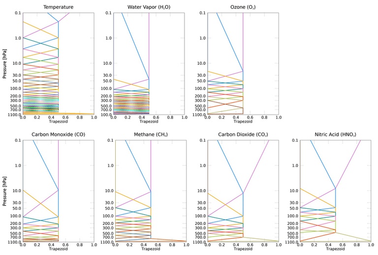
CLIMCAPS calculates Jacobians (weighting functions), not on the standard 100 retrieval pressure layers (air_pres_lay), but on a reduced set of overlapping pressure layers, referred to as trapezoid state functions. The use of trapezoid state functions was first developed by (Susskind et al., 2003) and remains a key feature of CLIMCAPS (Smith and Barnet, 2019, 2020) and AIRS V6 (Susskind et al., 2014) today.

The set of trapezoid state functions is unique to each retrieval variable. In Table 1 we list the relevant CLIMCAPS product fields, the number of state functions per variable as well as the upper and lower pressure layer values (i.e., the mid-point of the trapezoid ‘face’). Variables for which the radiance measurements have a higher (lower) information content, have more (fewer) state functions. The number of trapezoid state functions define the number of Jacobians and thus the dimension of the AK matrix for each retrieval variable. The full set of trapezoid state functions are visually depicted for seven retrieval variables in Figure 4.

Value of trapezoid state functions and how do they work in practice

Trapezoids greatly speed up Optimal Estimation retrievals with fewer calls to the forward model. All forward model calculations in CLIMCAPS are performed on the standard 100 pressure layers, but the Jacobians are calculated on the trapezoid state functions as brute force perturbation of the a-priori profiles (See Eq. 2 in Smith and Barnet 2020). Each a-priori profile is perturbed on multiple pressure layers at once according to the shape and magnitude of a trapezoid state function. For air_temp, CLIMCAPS calls the Stand-alone AIRS Radiative Transfer Algorithm (SARTA; Strow et al., 2003) 30 times, not 100 times, and for O₃, only nine times. Moreover, storing AK matrices on trapezoid pressure layers instead of the 100 retrieval layers significantly reduces CLIMCAPS product size. This is especially important for a global product across decades.

The AIRS science team determined the shape and distribution of trapezoids empirically to more closely represent the real information content of the measurements. Even though retrievals are reported on 100 levels (or layers) the number of levels (layers) the measurements have information content for is much less.

Table 1: Summary of CLIMCAPS averaging kernel variables in the product file. 

Retrieval Variable	Averaging kernel matrix [ave_kern/]	Trapezoid state function hinge-points [ave_kern/]	Number of trapezoid state functions	Ptop [hPa]	Pbot [hPa]
Air_temp	air_temp_ave_kern	air_temp_func_indxs	30	0.08	1056.4
H2O_vap	h2o_ave_kern	h2o_func_ indxs	21	5.5	1056.4
O3	o3_ave_kern	o3_func_indxs	9	2.9	822.6
CH4	ch4_ave_kern	ch4_func_indxs	11	1.7	943.4
CO	co_ave_kern	co_func_indxs	9	1.5	999.3
CO2	co2_ave_kern	co2_func_indxs	8	1.9	888.8
HNO3	hno3_ave_kern	hno3_func_indxs	8	1.3	733.92

Table note: All fields listed here are from the ave_kern/ group inside the netCDF file. P_top is the pressure layer value [hPa] of the top-most Trapezoid state function, and P_bot, the pressure layer value of the bottom-most state function. We read P_top and P_bot from the corresponding *_func_pres fields.

Each CLIMCAPS product file has a vector in the ave_kern netCDF group that defines the trapezoid pressure hinge-points (or indices) as the upper and lower limits of the trapezoid ‘face’. These are the *_func_indxs fields (Table 1, column 3).

Each variable has two additional fields that define their structure, namely *_func_hbot, and *_func_htop. A value of 1 indicate that the top trapezoid state function (i.e., the one that is closest to the top of atmosphere) is a trapezoid, whereas a value of 0 indicate that it is a wedge (Figure 10). Air_temp, CO₂ and HNO₃ all have *_func_htop = 0. CH₄, CO₂ and HNO₃ all have *_func_hbot = 0. These values become useful in the procedures we discuss below.

Figure 10: Trapezoid state functions for air_temp, H₂O_vap, O₃, CO, CH₄, CO₂ and HNO₃, which define the pressure levels on which CLIMCAPS Jacobians (weighting functions) and thus their averaging kernels are calculated.

Note how the trapezoid state functions overlap. This is to mimic correlation across vertical layers, and avoid introducing spurious structure in the retrieved profiles.

3. Convolving a reference profile

3.1 What are averaging kernels and how to use them

We distinguish two scenarios where averaging kernels may have value in applications:

• Inter-comparison studies using data in their native formats, without the need to convert to a common framework. In such cases, CLIMCAPS AKs on their trapezoid layers as distributed in the product file is sufficient to characterize information content and diagnose retrieval uncertainty on a scene-to-scene basis. We give examples of how this can be done with CLIMCAPS AKs in Smith and Barnet (2020). Iturbide-Sanchez et al., (2017) give another example using NUCAPS AKs (a CLIMCAPS sister algorithm).

• Applications, such as data assimilation and validation, may require measurements to be defined within a common framework that includes transforming them to the same vertical grid and applying similar smoothing constraints. We refer to this data transformation as ‘data convolution’. A typical example is the validation of retrieved soundings using radiosondes that were convolved using the retrieval’s AKs as outlined in Maddy and Barnet (2008). In simple terms, two types of ‘convolutions’ exist; Eq. 1 shows an example where a reference profile is smoothed according to the retrieval’s averaging kernel, or vertical resolution; Eq. 2 is the similar to Eq. 1 but additionally combines the reference profile with the retrieval a-priori.

Eq. 1          \(\widetilde{x}=\mathbf{F}_{Lj}^T\mathbf{A}_{LL}\mathbf{F}_{Lj}^+(x)\)

Eq. 2          \(\widetilde{x}=\ x_a+\mathbf{F}_{Lj}^T\mathbf{A}_{LL}\mathbf{F}_{Lj}^+\left({x-x}_a\right)\)

Where \(x\) [j × 1] is the reference profile (colloquially referred to as the ‘truth’ profile) from a different source, such as a radiosonde or reanalysis model profile interpolated to the standard 100 level retrieval grid, \(\widetilde{x}\) [j × 1] is the solution or convolved reference profile, \(x_{a}\) [j ×1] the CLIMCAPS a-priori profile (e.g., MERRA2 interpolated in time, space and pressure to match CLIMCAPS retrieval scenes and vertical grid),  F [L × j] is the transformation matrix reconstructed from the hinge-points, F⁺ [L × j] is the pseudo inverse of F, and A [L × L] is the averaging kernel matrix on trapezoid layers. Index L indicates the coarse vertical grid as defined by the trapezoid state function layers above surface pressure and j indicates the standard 100 retrieval levels above surface pressure. For gases, the linearity of Eq. 1 and Eq. 2 is achieved by using the log-form of the profiles, such that:

Eq. 3          \(\widetilde{x}=\ Exp[{\log(x}_a)+\mathbf{F}_{Lj}^T\mathbf{A}_{LL}\mathbf{F}_{Lj}^+\times\left({\log(x)-\log(x}_a)\right)]\)

We can refer to the matrix \( \mathbf{F}_{Lj}^T\mathbf{A}_{LL}\mathbf{F}_{Lj}^+ \) [j × j] as the effective averaging kernels of the 100-level retrieval profiles that describe the vertical correlation in the retrieval products, and thus their vertical resolution (Maddy and Barnet, 2008). If you wish to use CLIMCAPS averaging kernels on the 100 retrieval levels, then you need to calculate \( \mathbf{F}_{Lj}^T\mathbf{A}_{LL}\mathbf{F}_{Lj}^+ \) following the instructions below.

The averaging kernel matrix, A [L × L] is available for seven CLIMCAPS retrieval variables in the netCDF file as ave_kern/*_ave_kern (Table 1; Figure 1). The a-priori profiles for three retrieval variables are available in the CLIMCAPS product file as aux/fg_o3_mol_lay, aux/fg_h2o_vap_mol_lay and aux/fg_air_temp.

The a-priori profiles for CO, CO₂ and CH₄ should be calculated offline as detailed in the respective application guides. The only missing component is the calculation of the transformation matrix, F_Lj (using the pressure hinge-points as recorded in the ave_kern/*_func_indxs product field) and its inverse,  as:

Eq. 4          \(\mathbf{F}_{Lj}^+=[F_{Lj}F_{Lj}^{T}]^{-1}F_{Lj} \)

We demonstrate how to calculate F and F⁺ using pseudocode in Section 3.3.

3.2 Convolving radiosondes/ozonesondes to CLIMCAPS retrievals

A common practice is to convolve radiosondes and ozonesondes to satellite sounding retrievals to ease interpretation in some applications. Sondes have much higher vertical resolution, vertical sampling and vertical structure, compared to satellite soundings. Inter-comparisons can become difficult without convolving the higher-resolution measurement to the lower-resolution one because differences may be due to variation in quality or may be more reflective of their fundamental measurement characteristics. We will illustrate this with an ozonesonde as example.

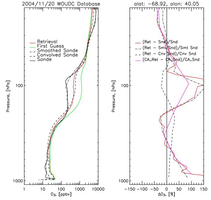
In Figure 11, left panel, there are five profiles; the ozone ‘sonde’ (solid black), the ‘retrieval’ (solid red) and the retrieval ‘first guess’, or a-priori (solid green). Applying Eq. 1 results in the ‘smoothed sonde’ (dash-dot-dash) and Eq. 2 in the ‘convolved sonde’ (dash-dash). We see here that the ‘sonde’ depict more vertical structure with a sharper tropopause transition.

The ‘retrieval’, in contrast, has less vertical structure with a smoother transition from troposphere to stratosphere. The retrieval improved upon its ‘first guess’ (which clearly over-estimated the upper troposphere lower stratosphere, UTLS, O₃ concentrations) but not enough to align with the ‘sonde’.  The ‘smoothed sonde’ has a smoother appearance, when compared to the original ‘sonde’ and the ‘convolved sonde’ aligns with the ‘retrieval’ because it is weighted by the ‘first guess’.

Figure 11: Demonstrating the value of convolving methods. Originally presented by Chris Barnet.

In Figure 11, right panel, we depict the percent bias and note how the convolved sonde bias as ‘(Ret – Cnv Snd)/Cnv Snd’ (dash-dash) oscillate around zero throughout the vertical column, and the smoothed sonde bias ‘(Ret – Smt Snd)/Smt Snd)’ (dash-dot-dash) has high peaks in the lower troposphere and UTLS. The convolved sonde statistics show us that the bias in the retrieval comes from the a-priori, not the radiance measurements or retrieval method.

3.3 Methodology – constructing the transformation matrix and its inverse

By ‘transformation matrix’, F, we mean the reconstructed trapezoid state functions as an [L × j] matrix that transforms the averaging kernel matrix [L × L] from course layers (L, Table 1) to the standard 100 pressure grid (j) as follows: \(\mathbf{F}_{Lj}^T\mathbf{A}_{LL}\mathbf{F}_{Lj}^+\) with dimension [j × j].

Four product fields are necessary to calculate the trapezoid state functions. They are the (1) 100-level pressure grid (air_pres), (2) shape of the top-most state function (ave_kern/*_func_htop), (3) shape of the bottom-most state function (ave_kern/*_func_htop), and (4) trapezoid state function indices (ave_kern/*_func_indxs).

As shown in Table 1, each variable has a different number of indices. The trapezoid state function indices (also known as hinge points), range in value between 1 and 100, each representing a pressure level in air_pres. When you reconstruct the trapezoid state functions using these hinge-points, they will resemble those in Figure 10.

We refer the reader to two IDL routines – slb2fin.pro that is called by calc_finv.pro. These routines are available as a standalone IDL procedures in our GitHub repository (https://github.com/climcaps), and we also appended them to the end of this chapter. In Table 2 and its discussion below, we attempt to clarify slb2fin.pro and demonstrate how it creates a trapezoid state function using the hinge points [ave_kern/*_func_indxs] available in the CLIMCAPS product file.

Table 2: A summary of the output created by slb2fin.pro for a single trapezoid state function.

Row num	Input parameters
	o3_func _indxs	air_pres [hPa]	func _ampl	IDL index, n	state _func	idx _down	idx _up	state _up	State _down	slope
1	1	0.04	0.0	0	0.0	0	25	0.0	0.0	0.0
2	26	23.45	0.0	1	0.0	25	34	0.0	0.0	0.0
3	35	56.13	0.0	2	0.5	34	38	0.0	0.5	1.53
4	39	77.24	1.0	3	0.5	38	43	0.5	0.5	0.0
5	44	110.24	0.0	4	0.0	43	48	0.5	0.0	-1.55
6	49	151.27	0.0	5	0.0	48	55	0.0	0.0	0.0
7	56	223.44	0.0	6	0.0	55	62	0.0	0.0	0.0
8	63	314.14	0.0	7	0.0	62	79	0.0	0.0	0.0
9	80	617.51	0.0	8	0.0	79	99	0.0	0.0	0.0
10	100	1100.00	0.0

Table notes: Here we use CLIMCAPS O₃ as example and list the content of [ave_kern/o3_func_indxs] in column 2. The standard 100-level pressure array [air_pres] in hPa units is listed in column 3. All other column titles refer to the variable names as used in slb2fin.pro and calc_finv.pro. Column 4 (‘func_ampl’) is defined in calc_finv.pro and used as one of the input variables to slb2fin.pro, and indicates that the fourth O₃ trapezoid state function should be calculated (row 4 of column 4 = 1.0).  The last column (‘slope’) defines the shape of the state function.

slb2fin.pro outputs the variable ‘func_fine’ with dimension [100]. This function corresponds to the fourth (from the top) O₃ trapezoid state function as depicted in Figure 10. When we look again at Table 1, we see that the trapezoid state function has a slope of 1.53 from pressure level index 35 to 39, then it has zero slope from pressure index 39 to 44 (this is the face of the trapezoid function) and a slope of -1.55 from pressure index 44 to 49.

The calc_finv.pro demonstrates how to implement Eq. 4 using IDL built-in routines.

IDL Routines

PRO slb2fin, numfunc, func_indx, func_apml, usehalftop, usehalfbot, presbot, air_pres, $ func_fine
; -------------------------------------------------
; PURPOSE: construct a trapezoid state function on 100 pressure levels
;          one at a time, using [ave_kern/*_func_indxs] hinge points
; -------------------------------------------------
; INPUT:
;  NAME            DESCRIPTION
; ----------    -------------------------
; numfunc        number of trapezoid state functions above Earth surface at retrieval scene
; func_indx      index values for trapezoid hinge points, starting at 1
; func_ampl      amplitude of trapezoids, which is 1.0 for the
; usehalftop     0 is a trapezoid, 1 is a wedge
; usehalfbot     0 is a trapezoid, 1 is a wedge
; presbot        pressure [hPa] of bottom retrieval level = 1100.0      
; air_pres        100-level retrieval pressure grid [air_pres]/100. in [hPa]

; OUTPUT:
; func_pfine    trapezoid state function on standard pressure level grid
;
;
; THIS FUNCTION IS CALLED BY CALC_FINV_MP.PRO
;
; ----------------------------------------------------------
; Step 1: Construct the face of the trapezoid state function
; ----------------------------------------------------------
      state_face = fltarr(numfunc)

      IF(usehalftop GT 0) THEN BEGIN
         state_face(0) = 0.5 * func_ampl(0)
      ENDIF ELSE BEGIN
         state_face(0) = func_ampl(0)
      ENDELSE

      FOR n = 1, numfunc-2 DO BEGIN
         state_face(n) = 0.5 * (func_ampl(n) + func_ampl(n-1))
      ENDFOR

      IF (usehalfbot GT 0) THEN BEGIN
         state_face(numfunc-1) = 0.5 * func_ampl(numfunc-2)
      ENDIF ELSE BEGIN
         state_face(numfunc-1) = func_ampl(numfunc-2)
      ENDELSE
; ---------------------------------------------------------------
; Step 2: Calculate the state function on standard 100 level grid
; ---------------------------------------------------------------
      FOR n = 0, numfunc-2 DO BEGIN
         idx_up = func_indx(n)-1
         idx_down = func_indx(n+1) - 1

         state_up = state_face(n)
         state_down = state_face(n+1)

         pres_up = alog(air_pres(idx_up))
         pres_down = alog(air_pres(idx_down))

         slope = (state_down - state_up)/(pres_down - pres_up)

         FOR L = idx_up, idx_down-1 DO BEGIN
            func_fine(L) = state_up + slope * (alog(air_pres(L)) - pres_up)
         ENDFOR
      ENDFOR

      func_fine(idx_down) = pres_down
END

PRO calc_finv_mp, num_func, func_indx, ret_nlev, htop, hbot, air_pres, $
      f_matrix, f_inv
; ---------------------------------------------
; PURPOSE: calculates a scene-dependent transformation matrix (F_matrix) and
;          its inverse the using Moore-Penrose pseudoinverse technique 
;          This matrix is scene-dependent because we use only those functions 
;          and pressure levels that are above Earth surface at target scene.

; INPUT:
;  Name          Description
; ---------    ----------------------
; num_func      number of state functions above Earth surface
; func_indx     trapezoid state function hinge-points
; ret_nlev      number of pressure levels (air_pres) above Earth surface 
; htop          value in [ave_kern/*_func_hbot]
; hbot          value in [ave_kern/*_func_htop]
; air_pres      standard 100 level pressure grid [air_pres]/100 in hPa units

; OUTPUT:
; f_matrix     transformation matrix where each retrieval state function is
;              on the standard retrieval pressure grid     
; f_inv        pseudoinverse matrix of f_matrix
;
; -----------------------------------------------------
; Step 1: calculate the transformation matrix: f_matrix
; -----------------------------------------------------
   num_func = num_func_indx-1
   f_matrix = FLTARR(num_func, ret_nlev)
   FOR ifunc = 0, nfunc - 1 DO BEGIN
;  Call slb2fin for one state function at a time setting the corresponding
;  slbval = 1.0
      slbval = FLTARR(num_func)
      slbval(ifunc) = 1.0
      fine = FLTARR(ret_nlev)
      SLB2FIN, num_func_indx, func_indx, slbval, htop, hbot, $
                   1100., air_pres, fine
      f_matrix(ifunc,*) = fine
   ENDFOR
; ------------------------------------------------
; Step 2: calculate the inverse of f_matrix using
;         the Moore-Penrose pseudoinverse method
; ------------------------------------------------
   fftr = MATRIX_MULTIPLY(DOUBLE(f_matrix),DOUBLE(f_matrix),/BTRANS)
   status=1L
   finv1 = LA_INVERT(fftr,STATUS=status,/DOUBLE)
   f_inv = MATRIX_MULTIPLY(finv1,DOUBLE(f_matrix))
END

 

4. References

• Clerbaux, C., Hadji-Lazaro, J., Hauglustaine, D., Mégie, G., Khattatov, B. and Lamarque, J.-F.: Assimilation of carbon monoxide measured from satellite in a three-dimensional chemistry-transport model, Journal of Geophysical Research: Atmospheres, 106(D14), 15385–15394, doi:10.1029/2000JD900682, 2001.
• Gaudel, A., Cooper, O. R., Ancellet, G., Barret, B., Boynard, A., Burrows, J. P., Clerbaux, C., Coheur, P.-F., Cuesta, J., Cuevas, E., Doniki, S., Dufour, G., Ebojie, F., Foret, G., Garcia, O., Granados-Muñoz, M. J., Hannigan, J. W., Hase, F., Hassler, B., Huang, G., Hurtmans, D., Jaffe, D., Jones, N., Kalabokas, P., Kerridge, B., Kulawik, S., Latter, B., Leblanc, T., Le Flochmoën, E., Lin, W., Liu, J., Liu, X., Mahieu, E., McClure-Begley, A., Neu, J. L., Osman, M., Palm, M., Petetin, H., Petropavlovskikh, I., Querel, R., Rahpoe, N., Rozanov, A., Schultz, M. G., Schwab, J., Siddans, R., Smale, D., Steinbacher, M., Tanimoto, H., Tarasick, D. W., Thouret, V., Thompson, A. M., Trickl, T., Weatherhead, E., Wespes, C., Worden, H. M., Vigouroux, C., Xu, X., Zeng, G., Ziemke, J., Helmig, D. and Lewis, A.: Tropospheric Ozone Assessment Report: Present-day distribution and trends of tropospheric ozone relevant to climate and global atmospheric chemistry model evaluation, Elem Sci Anth, 6, doi:10.1525/elementa.291, 2018.
• Iturbide-Sanchez, F., Liu, Q., Gambacorta, A., Barnet, C., Nalli, N. R., Tan, C. and Santos da Silva, S. R.: Using averaging kernels to study the vertical resolution of nucaps temperature and water vapor, in 2017 IEEE International Geoscience and Remote Sensing Symposium (IGARSS), pp. 33–35, IEEE, Fort Worth, TX., 2017.
• Levelt, P. F., Khattatov, B. V., Gille, J. C., Brasseur, G. P., Tie, X. X. and Waters, J. W.: Assimilation of MLS ozone measurements in the global three-dimensional chemistry transport model ROSE, Geophysical Research Letters, 25(24), 4493–4496, doi:10.1029/1998GL900152, 1998.
• Liu, J., Fung, I., Kalnay, E., Kang, J.-S., Olsen, E. T. and Chen, L.: Simultaneous assimilation of AIRS Xco ₂ and meteorological observations in a carbon climate model with an ensemble Kalman filter: ASSIMILATION OF AIRS XCO ₂, Journal of Geophysical Research: Atmospheres, 117(D5), n/a-n/a, doi:10.1029/2011JD016642, 2012.
• Maddy, E. S. and Barnet, C. D.: Vertical Resolution Estimates in Version 5 of AIRS Operational Retrievals, IEEE Transactions on Geoscience and Remote Sensing, 46(8), 2375–2384, doi:10.1109/TGRS.2008.917498, 2008.
• Maddy, E. S., Barnet, C. D. and Gambacorta, A.: A Computationally Efficient Retrieval Algorithm for Hyperspectral Sounders Incorporating A Priori Information, IEEE Geoscience and Remote Sensing Letters, 6(4), 802–806, doi:10.1109/LGRS.2009.2025780, 2009.
• Nalli, N. R., Barnet, C. D., Reale, A., Tobin, D., Gambacorta, A., Maddy, E. S., Joseph, E., Sun, B., Borg, L., Mollner, A. K., Morris, V. R., Liu, X., Divakarla, M., Minnett, P. J., Knuteson, R. O., King, T. S. and Wolf, W. W.: Validation of satellite sounder environmental data records: Application to the Cross-track Infrared Microwave Sounder Suite: SATELLITE SOUNDER EDR VALIDATION, Journal of Geophysical Research: Atmospheres, 118(24), 13,628-13,643, doi:10.1002/2013JD020436, 2013.
• Pierce, R. B., Al-Saadi, J., Kittaka, C., Schaack, T., Lenzen, A., Bowman, K., Szykman, J., Soja, A., Ryerson, T., Thompson, A. M., Bhartia, P. and Morris, G. A.: Impacts of background ozone production on Houston and Dallas, Texas, air quality during the Second Texas Air Quality Study field mission, Journal of Geophysical Research, 114, doi:10.1029/2008JD011337, 2009.
• Rodgers, C. D.: Inverse methods for atmospheric sounding: theory and practice, World Scientific, Singapore; Hackensack, N.J., 2000.
• Rodgers, C. D. and Connor, B. J.: Intercomparison of remote sounding instruments: INTERCOMPARISON OF REMOTE SOUNDERS, Journal of Geophysical Research: Atmospheres, 108(D3), n/a-n/a, doi:10.1029/2002JD002299, 2003.
• Segers, A. J., Eskes, H. J., van der A, R. J., van Oss, R. F. and van Velthoven, P. F. J.: Assimilation of GOME ozone profiles and a global chemistry–transport model using a Kalman filter with anisotropic covariance, Quarterly Journal of the Royal Meteorological Society, 131(606), 477–502, doi:10.1256/qj.04.92, 2005.
• Smith, N. and Barnet, C. D.: Uncertainty Characterization and Propagation in the Community Long-Term Infrared Microwave Combined Atmospheric Product System (CLIMCAPS), Remote Sensing, 11(10), 1227, doi:10.3390/rs11101227, 2019.
• Smith, N. and Barnet, C. D.: CLIMCAPS Observing Capability for Temperature, Moisture and Trace Gases from AIRS/AMSU and CrIS/ATMS, Atmospheric Measurement Techniques, 13, 4437–4458, doi:10.5194/amt-13-4437-2020, 2020.
• Strow, L. L., Hannon, S. E., De Souza-Machado, S., Motteler, H. E. and Tobin, D.: An overview of the AIRS radiative transfer model, IEEE Transactions on Geoscience and Remote Sensing, 41(2), 303–313, doi:10.1109/TGRS.2002.808244, 2003.
• Susskind, J., Barnet, C. D. and Blaisdell, J. M.: Retrieval of atmospheric and surface parameters from AIRS/AMSU/HSB data in the presence of clouds, IEEE TGRS, 41, 390–409, 2003.
• Susskind, J., Blaisdell, J. M. and Iredell, L.: Improved methodology for surface and atmospheric soundings, error estimates, and quality control procedures: the atmospheric infrared sounder science team version-6 retrieval algorithm, Journal of Applied Remote Sensing, 8(1), 084994, doi:10.1117/1.JRS.8.084994, 2014.
• Yudin, V. A.: Assimilation of the 2000–2001 CO MOPITT retrievals with optimized surface emissions, Geophysical Research Letters, 31(20), doi:10.1029/2004GL021037, 2004.