Background

CLIMCAPS uses Quality Control (QC) metrics to intuitively communicate which vertical and spatial observations of temperature (T(p)), water vapor (H₂O), and trace gases are appropriate to use. We will describe how to access, interpret, and use the QC flags inside the CLIMCAPS netCDF file.

1. Vertical Quality Control Flags

In the CLIMCAPS netCDF file, users can access the QC metrics in the fixed pressure grid for each of the retrieved and derived variables by accessing fields that end in *_qc. CLIMCAPS defines retrievals as successful if all steps of the retrieval successfully executed; if any steps do not pass or if they fail any additional internal quality checks, then the retrieval is flagged as having failed.

All variables inside the netCDF file that end in *_qc have the exact same values because CLIMCAPS V2 employs a single QC schema for all retrieval variables. CLIMCAPS being a step-wise retrieval procedure, we argue that if T(p) fails, then all subsequent retrieval variables should also be flagged as failed. For example, CO_mol_lay_qc has identical values to those in the O3_mol_lay_qc variable. In the future, we may consider adopting variable-specific QC flags, so we recommend using the variable-specific QC flag in your code. For example, if you are working with CO_mol_lay, then use the CO_mol_lay_qc variable.

The QC flag has three possible values, which are 0, 1, and 2. To improve understanding of QC, we encourage users to interpret these respective values as best, good, and rejected (Table 1).

Note that in addition to the *_qc variables, there are error (*_err), degrees of freedom (*_dof), and averaging kernel matrix variables inside the netCDF file, which are also important indicators of quality and information content.

Table 1: Description of quality control values and their appropriate use

Value	Meaning	Appropriate Use
0	Best	Best QC retrievals can be used without reservation following the guidance of the variable-specific application guides. We recommend that users develop a general understanding of the available information content of the variable to ensure they are appropriately interpreting atmospheric state variables. Best QC retrievals can be used for in situ measurement comparison, data assimilation, or another research application.
1	Good	When combined with the best QC retrievals, good QC retrievals increase the yield of available profiles and thus are useful for applications that require a large sample of retrievals. Good QC retrievals are appropriate for applications where measurements are spatially or temporally aggregated. It is recommended that users analyze good retrievals alongside measures of variable information content, which includes degrees of freedom (DOF; *_dof) and the Averaging Kernel Matrix (AKM; ave_kern/*_ave_kern), and errors (*_err). These are described in detail in variable-specific application guides.
2	Rejected	We do not recommend using rejected retrievals unless the region is data sparse. These are cases where it may be more appropriate to use the CLIMCAPS MW-only retrievals (mw/mw_air_temp, mw/mw_h2o_vap_mol_lay). If using IR+MW retrievals, it is strongly recommended that rejected retrievals are analyzed alongside measures of information content, which include DOFs, AKMs, and errors. Additionally, rejected retrievals should also be evaluated in context of cloud clearing parameters (aux/etarej, aux/ampl_eta, and aux/aeff_end), which are described later in this user guide.

Global and zonal yield of QC by height

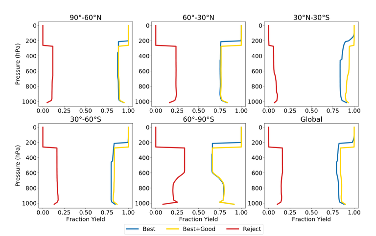
Figure 1 illustrates the global and zonal yield of QC by height. Measurements that are below the surface pressure are not included in Figure 1 or the discussion below. However, note that measurements below the surface will automatically have a QC flag value of 2 (rejected) in the netCDF file. We calculated our yield fraction by dividing the number of observations with a specific quality flag with the total number of observations at the given pressure level.

Clouds are one of the primary reasons why retrievals fail. For this reason, retrievals in the stratosphere have a much higher yield than in the troposphere, which is reflected in the sharp discontinuity above the tropopause of each zone.

Across all zones, the yield is nearly 1.0 above 200 hPa for ‘best’ and the combined ‘best’ and ‘good’ (best+good) quality retrievals. There is greater variability between 1000 hPa and 800 hPa across each of the latitude zones shown in Figure 1. For example, the lowest yield occurs in the southern polar region (60°S-90°S), which between 600-200 hPa has a rejection rate of 0.30. Combing ‘best’ and ‘good’ retrievals increases the yield significantly in the tropics (30°N-30°S).

Figure 1: Fraction of retrievals with a given QC flag for CLIMCAPS-SNPP T(p) retrievals (air_temp_qc) from full spectral resolution cloud cleared CrIS radiances. The results are shown for five latitudinal zones and for the full global retrieval. ‘Best’ quality data has a QC flag value of 0, ‘best+good’ has a value of 0 or 1, and rejected data has a value of 2. Note that while each variable has a corresponding *_qc field, these values do not vary between CLIMCAPS state and derived variables. The example presented here is from CLIMCAPS-SNPP retrievals on 1 April 2016.

2. Footprint Quality Control

Users may also wish to use a single QC metric for the entire footprint, rather than by pressure level. For this application, we recommend the QC approach adopted by the NOAA-Unique Combined Atmospheric Processing System (NUCAPS) for the National Weather Service (NWS) that we summarized in this quick-guide. NUCAPS is a sister algorithm to CLIMCAPS, specifically designed for real-time monitoring of hazardous weather.

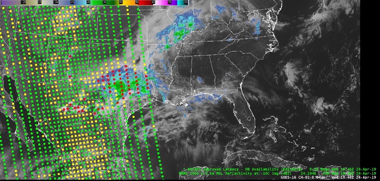
This NUCAPS QC method was developed to facilitate forecaster interpretation during severe weather events and uses a visually intuitive, “stoplight” color coding approach. In this method, footprints are labeled green when both microwave and infrared retrievals pass (clear sky/partly cloudy conditions), yellow when the MW-only passes (cloudy conditions), and red when both the combined IR+MW and the MW-only steps fail (precipitating conditions).

An example of this QC method is shown in Figure 2, which shows a screen capture of NUCAPS NOAA-20 from the NWS AWIPS-II visualization software.

Figure 2: Example of a footprint-level QC approach used in the NUCAPS algorithm by the National Weather Service (NWS). Green retrievals indicate the IR+MW step successfully passed, yellow retrievals where the MW-only step passed while the IR+MW step failed, and red indicates both steps were rejected. The example is taken from a screen capture from AWIPS-II of NUCAPS from a NOAA-20 overpass of convection at 19:45 UTC on April 24, 2019.

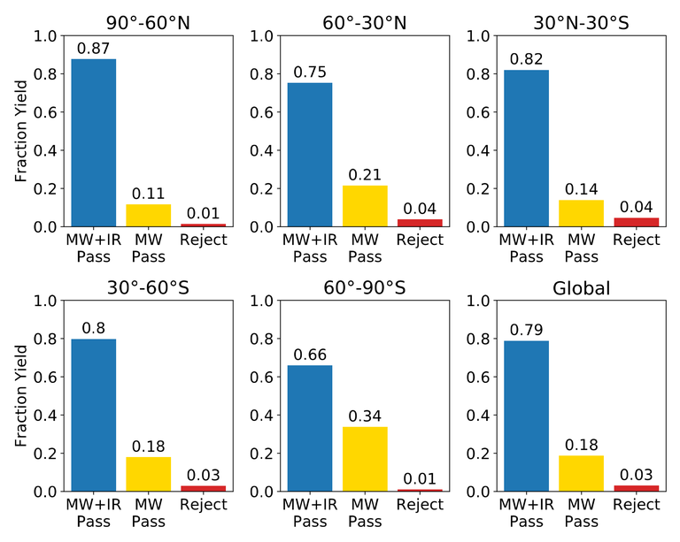
The NUCAPS single footprint QC method can also be implemented in CLIMCAPS by reading the aux/ispare_2 in the netCDF file. Figure 3 shows the zonal yield fraction for each of these QC flags.

Using the NUCAPS QC method, the highest yield (0.87) of retrievals where MW+IR passed is in the northern polar region (90°N−60°N) and lowest yield (0.66) is in the southern polar region (60°S−90°S). Globally, the percent yield is roughly 0.80, with only a 0.03 rate of rejection.

Figure 3: Fraction of retrievals with a given QC flag for CLIMCAPS-SNPP T(p) retrievals (aux/ispare_2) from full spectral resolution cloud cleared CrIS radiances. The results are shown for five latitudinal zones and for the full global retrieval. ‘MW+IR Pass’ data has a bit flag of zero, ‘MW-only Pass’ has a value of 1, and ‘Reject’ has a value of 9. Results presented here are for CLIMCAPS-SNPP retrievals on 1 April 2016.

The values inside the aux/ispare_2 field have three values: 0, 1, and 9, which correspond to MW+IR Pass, MW Pass, and Reject. These numbers are not sequential because they are encoded as 8-bit binary values to diagnose which components of the retrieval failed or succeeded. However, the values can be read as integers and do not need to be read bitwise in order to interpret their meaning.

3. Data filtering options

In addition to quality flags, users may wish to filter CLIMCAPS footprints by time of day or scene type, such as during sunlight, over land or ocean, and clear or cloudy scenes. Furthermore, users may wish to filter the vertical measurements into the troposphere or stratosphere. Below, we include some data filtering options based on options that are available in the CLIMCAPS Level 2 product file. Note that for all options below, i and j respectively refer to the footprint indices along the atrack and xtrack.

Ascending versus Descending

• asc_flag(atrack) The ascending flag is useful for determining whether a granule is from an ascending or descending orbit. If asc_flag(i) = 1 then the retrieval is from the ascending orbit, which means it has a 01:30 pm local overpass time. If asc_flag(i) = 0 then the retrieval is from the descending orbit and thus at the 01:30 am local overpass time.
• lat(atrack,xtrack) Changes in latitude between scanlines is also a helpful indicator of the orbit direction. If lat(i+1,j) > lat(i,j) then the granule is in ascending (01:30 pm) orbit and if lat(i+1,j) < lat(i,j) then granule is in the descending (01:30 am) orbit.

Sun versus No Sun

• sol_zen(atrack,xtrack) The solar zenith angle is a function of latitude, the local time, and day of the year. The solar zenith angle is useful for determining if the sun is above or below the horizon at a specific location, thus it may be used to classify a footprint as being exposed to sunlight or not. For sol_zen(i,j) = 0, the sun is directly above the footprint, and for sol_zen(i,j) = 90 the sun is at the horizon at the time of satellite measurement. If sol_zen(i,j) > 90, then sun is below the horizon and thus have no impact on the radiance measurement or retrieval. In CLIMCAPS, we use a threshold of sol_zen(i,j) = 89.9˚ to determine if solar reflectivity should be accounted for or not.

Land versus Ocean

• land_frac(atrack,xtrack) The land fraction measures how much a footprint falls over land as opposed to water. For example, if land_frac(i,j) ≥ 0.75 (thus 75%) then the retrieval footprint is mostly over land. One can consider a range of 0.75 > land_frac(i,j) ≥ 0.25 (thus 25-75%) for a retrieval footprint to be over coastlines. If land_frac(i,j) < 0.25 (thus 25%) then the retrieval footprint is mostly over ocean. In CLIMCAPS V2 we do not distinguish between land or ocean during retrieval. Instead, for a footprint with mixed surface types, CLIMCAPS simply makes a weighted average (as determined by the fraction of each surface type) of the land and ocean emissivity spectra. In applications, you may wish to clearly distinguish land from ocean, so you may define your own land_frac thresholds.

Clear-sky versus Cloudy

• aux/for_cldfrac_tot(atrack, xtrack) The total cloud fraction over the retrieval footprint (3 x 3 fields of view; ~50 km at nadir, ~150 km at edge of scan). CLIMCAPS employs cloud clearing, which allows successful retrievals in up to 90% cloudy conditions. Your application may need to distinguish between clear and cloudy scenes, so you can use for_cldfrac_tot (i,j)> 0.10 (thus more then 10% cloud cover) as ‘cloudy’ and for_cldfrac_tot (i,j) ≤ 0.10 as ‘clear’. You can, of course, vary these values according to the requirements of your application.
• aux/cldfrac_500(atrack, xtrack) The total cloud fraction below 500 hPa over the retrieval footprint. This metric is useful for identifying scenes with lower tropospheric clouds.
• cld_frac(atrack, xtrack, fov, cld_lay) Like aux/cldfrac_tot, cld_frac is the total cloud fraction but instead it is over the instrument field of view (using the fov index) and not the CLIMCAPS footprint (3 x 3 FOVs). cld_frac is available as two cloud layers using the cld_lay index, where cld_lay = 1 is the lower cloud layer and cld_lay = 2 is the upper cloud layer over the instrument field of view. The interpretation of the values is the same as that of aux/cldfrac_tot.
• aux/etarej(atrack, xtrack) Rather than inspect the cloud fraction, you may wish to filter retrievals based on cloud uncertainty. This metric is the cloud clearing radiance error in brightness temperature units [Kelvin]. CLIMCAPS calculates it as radiance residual, or the difference between the simulated clear-sky radiance estimate and the retrieved cloud cleared radiance at a retrieval scene. etarej, thus, quantifies the quality of cloud clearing by indicating how well the cloud-cleared radiance represents the clear-sky state around clouds. etarej is one of the QC criteria employed in determining whether a retrieval failed or not (using a threshold of 1.5K). Smaller values of etarej indicate successful cloud clearing and a high confidence in the removal of the radiance signal from clouds. Higher values of etarej indicate that cloud cleared radiance channels are ‘contaminated’ by cloud radiative effects that we were unable to remove during the cloud clearing step. We recommend that you use etarej to identify CLIMCAPS retrievals with cloud contamination, or uncertainty due to clouds.
• aux/ampl_eta(atrack, xtrack) The amplification factor (ampl_eta) quantifies how much the random instrument noise (NEN or NEdT in units Kelvin) was amplified (ampl_eta(i,j) > 1) or damped (ampl_eta(i,j) < 1) as a result cloud clearing.
• aux/aeff_end(atrack, xtrack) The effective amplification factor (aeff_end) is a compound metric that combines random instrument noise as scaled by the ampl_eta with systematic uncertainty due to spectral correlation.

Troposphere versus Stratosphere

• tpause_pres(atrac, xtrack) The tropopause pressure is useful for stratifying the troposphere from the stratosphere.