Definitions

Satellite soundings as profiles of temperature, T(p), water vapor (H₂O) and trace gases along a pressure grid [hPa], from the Earth surface to top of atmosphere. CLIMCAPS reports its retrieved soundings on the standard 100 level pressure grid also used in SARTA (Strow et al., 2003), which spans 1100 hPa to 0.016 hPa.

CLIMCAPS retrieves T(p) as the temperature at each pressure level, while it retrieves H₂O, O₃, CO, CH₄, HNO₃, N₂O and SO₂ (i.e., all gases except CO₂) as column densities [molec/cm²] on pressure layers (Section 1).

A pressure layer is the vertical area between two pressure levels. CLIMCAPS retrieves CO₂ as pressure layer mixing ratio [ppb], although CO₂ is reported in the product files as volume mixing ratio on pressure levels, which is the mole of CO₂ per mole of dry air [mol/mol].

In this document we discuss issues that can significantly affect data application and understanding as they relate to CLIMCAPS retrieval levels and layers. These are:

1. Levels versus Layers, and converting from one to the other.
2. Adjusting retrieved profiles to scene surface pressure

1. Levels versus Layers

CLIMCAPS requires all state variables to be on the standard 100 pressure levels used in SARTA (Strow et al., 2003) for accurate calculations of top of atmosphere infrared radiance in narrow spectral intervals. This is a fixed 100-level pressure grid (P_lev) and available in the CLIMCAPS product file as air_pres, which is the same at all scenes across the globe irrespective of variations in Earth surface pressure. P_lev(1) = 0.016 hPa, and P_lev(100) = 1100.0 hPa.

CLIMCAPS does not retrieve surface pressure but instead uses MERRA-2 surface pressure as state variable and write it to the product files as: aux/prior_surf_pres [Pa]. The MERRA-2 surface pressure values written to aux/prior_surf_pres [Pa] have been spatially and temporally interpolated to CLIMCAPS.

Over the ocean, surface pressure is typically 1013.25 hPa. High terrain surface pressure is often less than 800 hPa, such as over the Tibetan Plateau in Asia, the Rocky Mountains in North America, and the Andes Mountains in South America. Most of the time P_lev(100) is well below Earth surface pressure, which means that one needs to truncate the retrieved profiles according to the true Earth surface pressure at the target scene.

The CLIMCAPS product field, air_pres_lay_nsurf, contains the index where the standard air_pres array intersects Earth surface pressure (aux/prior_surf_pres) at a target retrieval scene. In each CLIMCAPS product file there is air_pres with dimension [air_pres] where air_pres = 100, and air_pres_lay_nsurf with dimension [atrack x xtrack], where atrack = 30 to indicate the number of retrieval footprints along each scanline and xtrack = 45 to indicate the number of scanlines per file.

Similarly, for the pressure layer array, air_pres_lay, there is a corresponding air_pres_lay_nsurf field. One should truncate temperature retrieval at position atrack = i and xtrack = j with P_bot = air_pres_lay_nsurf(i, j) such that T(p) = air_temp(i, j, 1:P_bot).

Stated differently, CLIMCAPS profile retrievals are valid from the top of atmosphere, air_pres(1), to the Earth surface as defined by MERRA-2 surface pressure (aux/prior_surf_pres) and indicated by air_pres_lay_nsurf for each retrieval scene

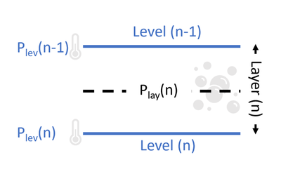
CLIMCAPS retrieves trace gas quantities on a standard pressure layer grid (air_pres_lay), which is a 100 layer grid derived from air_pres. Figure 1 gives a graphic representation of pressire levels versus layers. 

Figure 1: An illustration showing the differences between CLIMCAPS pressure levels (P_lev) [air_pres] and pressure layers (P_lay) [air_pres_nsurf] for an index n, where . Temperature is retrieved on levels while trace gasses are retrieved on pressure layers. The mathematical conversion from levels to layers is shown in Eq. 1.

We derive the pressure layer ( \( P_{lay} \) ) grid from pressure levels (\( P_{lev} \)) as follows:

Eq. 1          \( P_{lay} (n) = \frac{ P_{lev} (n) - P_{lev} (n-1) }{\log_{10}\big(P_{lev}(n)/P_{lev}(n-1)\big) } \)

where \(n \in \{2,...,100\} \), \(P_{lay}(1) = 0.00284 \) hPa, and \(P_{lay}(100) = 1085.36 \) hPa. All trace gas quantities in the mol_lay group, as well as aux/co2_vmr are retrieved and reported on this pressure layer grid. It is thus important that you associate the CLIMCAPS trace gas retrieval profiles with pressure layers (air_pres_lay) not levels (air_pres).

Converting Levels to Layers

Some applications may require you to evaluate CLIMCAPS temperature retrieval levels alongside H₂O density layers. In such cases, convert air_temp from its native definition on air_pres levels to air_pres_lay layers as follows:

Assume that the top of atmosphere temperature is isothermal (Eq. 2), while all other layers are calculated as two-point running means (Eq. 3).

Eq. 2          \( T_{lay}(n) = T_{lay}(n), n=1 \)

Eq. 3          \( T_{lay}(n) = 0.5 \times ( T_{lev}(n) + T_{lev}(n-1) ), n \in \{2,...,100\} \)

Converting Layers to Levels

If you wish to represent CLIMCAPS column density trace gas retrievals[molecules/cm²] on pressure levels, we recommend the procedure below. ­­Note that with this conversion from pressure layers to levels we will use water vapor column density (h2o_vap_mol_lay) as example in the pseudocode below.

2. Adjusting retrieved profiles to surface pressure at a target scene

CLIMCAPS retrieves atmospheric variables along a standard pressure grid that does not account for variation in surface pressure, P_s. The CLIMCAPS product file records the standard pressure level (air_pres) and pressure layer (air_pres_lay) array index closest to surface pressure P_s, as air_pres_lay_nsurf.

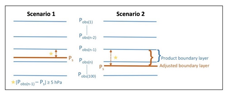
When the standard 100-level air_pres array intersects with Earth surface pressure at a target scene, one of two scenarios occur, which we demonstrate in Figure 2.

Figure 2: An illustration of the two types of boundary layer conditions that result when retrieving atmospheric variables on a standard pressure grid, P_obs, which for CLIMCAPS is the pressure levels profile, air_pres. CLIMCAPS uses surface pressure, P_s, from MERRA-2. Here the subscript n denotes ranges from 1 to 100, and represents the index at which the CLIMCAPS retrieval is reported at. Unless the retrieval is performed over ocean P_obs(n) is always less than P_obs(plev) with n < plev, plev = 100, and P_obs(plev) = 1100 mb. Scenario 1 requires a narrowing of the boundary layer with interpolation of the retrieved value from P_obs(n-1) to P_s. Scenario 2 requires a broadening of the boundary layer with extrapolation of the retrieved value from P_obs(n-1) to P_s. The brown dotted line indicates the width of the adjusted boundary layer, which always exceeds 5 mb and varies horizontally with surface topography.

We define surface air temperature (T_surf) as the atmospheric temperature at surface pressure (P_surf; aux/prior_surf_pres). We can derive T_surf from the retrieved temperature profile (air_temp) as follows:

Eq. 4          \( T_{surf} = T(P_{bot}-1) + BL_{mult} \times [ T(P_{bot}) - T(P_{bot}-1) ] \)

Where \(BL_{mult}\) is the boundary layer multiplier that quantifies the degree to which the bottom profile level needs to be adjusted so that the bottom temperature value represents the temperature at surface pressure, not the standard level closest to surface pressure. \(P_{bot}\) (air_pres_lay_nsurf) is the index of the pressure level that is closest to P_surf while always satisfying the condition:

Eq. 5          \( [ P_{surf}-P_{lev}(P_{bot}-1)] \geq 5 hPa \)

This condition ensures that P_lev(P_bot) is always less than P_surf by at least 5 hPa. BL_mult is given by:

Eq. 6          \( BL_{mult} = \frac{P_{surf} - P_{lev}(P_{bot}-1)}{P_{lev}(P_{bot})-P_{lev}(P_{bot}-1)} \)

Figure 2 Scenario 1 demonstrates a case where BL_mult < 1.0, and Scenario 2 a case where BLmult ≥ 1.0.

Eq. 3 convert temperature from level to a layer for any layer in the temperature profile. In context of surface layer, Eq. 4 can be used to calculate the bottom layer with:

Eq. 7          \( T_{lay}(P_{bot}) = 0.5 \times ( T(P_{bot}-1) + T_{surf} ) \)

For traces gases, the values are retrieved as layer column density, so the boundary layer column density should be adjusted for surface pressure P_surf differently than for air_temp on pressure levels. The boundary layer for trace gases is indicated by the P_bot (air_pres_lay_nsurf) of air_pres_lay. This bottom layer needs to be either narrowed (Figure 2, Scenario 1) or broadened (Figure 2, Scenario 2) with B_mult as follows:

Eq. 8          \( CD_{surf} = BL_{mult} \times T_{gas}(P_{bot}) \)

Where \(T_{gas} \) depicts any of the CLIMCAPS trace gas retrieval species, including CO₂.

The CLIMCAPS temperature retrieval product, air_temp, already has this correction applied, which means that air_temp(i,j,P_bot) is the temperature at surface pressure. 

The CLIMCAPS trace gas column densities, e.g., wat_vap_mol_lay, does NOT have this correction applied and you have to follow the instructions in Section 3 below to make the adjustment. 

All CLIMCAPS derived values, such as relative humidity and mixing ratio, has this correction applied, so you can use those fields as is. 

3. Pseudocode for adjusting boundary layer values

Calculating BL_mult 

Below, we show some example pseudocode to calculate BL_mult from Eq. 6. Three variables are required from the CLIMCAPS netCDF file: air pressure (air_pres), L_bot (air_pres_nsurf), and P_surf (aux/prior_surf_pres). P_surf is a two-dimensional variable (y (atrack), x (xtrack)). We simplify our discussion by only calculating BL_mult and T_surf at the first footprint (atrack = xtrack = 0).

Calculating T_surf

Below we show an example pseudocode to calculate T_surf, for a single footprint, which we showed in Eq. 4. We first import the T(p) variable (air_temp) from the netCDF file. T(p) is a three-dimensional variable (y (atrack), x (xtrack), and z (air_pres)), so like psurf in our BLmult pseudocode above, we keep only the value from the first footprint (atrack = xtrack = 0). The variable t_diff is the difference between the temperature from the level above the bottom level and the temperature from the level at Pbot. Surface temperature (t_surf) is then calculated on the last line.

The above code will map a single value to t_surf. To calculate T_surf over the entire swath, surface temperature can be defined as a two-dimensional vector. Instead of using the first footprint (atrack = xtrack = 0), the user can write a loop and iterate over atrack and xtrack to calculate the T_surf for all footprints in the file(s).

Calculating Total Water Vapor

Water vapor is often integrated to show column total H₂O. In our example pseudocode below, we import the H₂O column density (h2o_liq_mol_lay), and extract the column values for the first footprint (iobs = 0). Then, we compute total H₂O for all layers except the bottom layer, from 1 to P_bot-1. We adjust the bottom layer (P_bot) with BL_mult and add it to the total, as shown in Eq. 8. Like T(p), users can incorporate the procedure from the pseudocode below in a loop to process the whole swath.