Key Questions

CLIMCAPS retrieves profiles of atmospheric water (H₂O) vapor column densities (molec/cm²) on the standard 100 pressure layers using subsets of spectral channels from both infrared (IR) and microwave (MW) measurements. The IR set includes channels from the longwave band, 780–1090 cm⁻¹ (~9.2–12.8 μm), and midwave band, 1213–1745 cm⁻¹ (~5.7–8.2 μm), with a total of 66 channels for CrIS and 46 for AIRS. The MW set includes channels from the 89 GHz line for AMSU and the 165.5 GHz and 183.31 GHz lines for ATMS.

How can I access CLIMCAPS H₂O retrievals? 

CLIMCAPS H₂O retrievals are distributed within the main product file that is generated and archived by the NASA Goddard Earth Sciences Data and Information Services Center (GES DISC). 

Is there a way to quickly identify wet/dry regions for my application?

Yes. The CLIMCAPS netCDF file has a hierarchical structure to keep the fields organized according to type and application. The base level contains a few instrument and atmospheric variables that are easily accessible and frequently used in applications. Among them are three fields derived from the retrieved H₂O vapor column density. They are (i) h2o_vap_tot, or the total mass of water vapor content [kg/m²] more commonly referred to as total precipitable water (TPW) [mm] and, (ii) rel_hum/spec_hum, relative humidity [%] and specific humidity [kg/kg], respectively. Each of these fields have an associated quality control (qc) field, e.g., h2o_vap_tot_qc and you can use all values where qc is 0 or 1.  

Which retrievals should I avoid?

The short answer is that you should avoid all retrievals where the quality control (qc) associated with a target field, e.g., rel_hum_qc for rel_hum, is equal to 2. There is a qc value for each level, so if the target field is a profile on pressure layers defined by air_pres_h2o (66 levels) then there will be 66 x qc values for that profile that flags the vertical layers either as 0 (best quality), 1 (good quality) or 2 (bad quality).

There are two unusual cases that may affect your application since they are not necessarily flagged as ‘bad quality’ (qc = 2).

Cases of excessively dry layers

On rare occasions, CLIMCAPS H₂O retrieval profiles, specifically the netCDF fields spec_hum, rel_hum, and mol_lay/h2o_vap_mol_lay, have zero or unphysically low values in one or two pressure layers without being flagged as bad quality (qc = 2). These occur for two reasons: (1) due to MERRA2, the CLIMCAPS a-priori for H₂O, that contains extremely dry layers on the order of ~10⁻²⁰ kg/kg and, (2) due to numerical precision when the CLIMCAPS pre-processor converts these MERRA-2 profiles from their native 72 levels to the standard 100 retrieval layers (air_pres_lay) used in retrieval. We advise you to inspect these field and remove the entire profile where any layer value equals zero and your application is sensitive to this.  h2o_vap_tot is not affected.  

Cases of super saturation

We added a quality control filter in CLIMCAPS that rejects retrievals (sets qc = 2) whenever relative humidity exceeds 110% anywhere between the Earth surface and 300 hPa. At pressure levels above 300 hPa, super saturation is physically common due to the combination of low H₂O concentrations and cold temperatures. This rejection criteria reduces the number of global retrievals by about 5% globally. Your application may require a more stringent humidity threshold, so we recommend that you evaluate results and create your own filter to better suit your application if necessary.

1. Overview

1.1 Combined IR and MW H₂O retrieval

CLIMCAPS uses spectral channels from both MW (AMSU/ATMS) and IR (AIRS/CrIS) measurements to retrieve H₂O. By combining MW and IR, CLIMCAPS can achieve and maintain robust retrieval quality in both clear and partly cloudy scenes. The contribution each set of channels make to the final retrieval varies, since CLIMCAPS calculates scene-dependent information content and then weighs the spectral channels accordingly.

For instance, clouds are opaque in the IR and thus one of the main sources of noise (Smith and Barnet, 2019). Relative to cloudy scenes, IR measurements of clear scenes have low scene-dependent noise. In clear cases, CLIMCAPS will thus give a strong weight to IR channels so that they make a larger contribution to the final retrieval. MW, on the other hand, has lower scene-dependent noise due to clouds (for all but non-precipitating clouds), so in complex cloudy scenes where IR information content is lower, CLIMCAPS will give stronger weight to the MW channels in its temperature and H₂O retrievals. CLIMCAPS thus leverages the different sensitivities and skills of IR and MW measurements to stabilize and optimize its retrievals.

Rather than using all available channels, CLIMCAPS use subsets of channels most sensitive to the target retrieval variable (e.g., H₂O) and with minimal sensitivity to other interfering variables. The CLIMCAPS H₂O channel set from IR measurements (AIRS and CrIS) is centered on water lines in the midwave, 3.7 µm, 6.6 µm—and longwave, 12 µm—spectral regions. For MW, CLIMCAPS uses channels in the 89 GHz band for AMSU and the 165.5 GHz as well as 183.31 GHz bands for ATMS.

Despite careful channel selection, it is impossible to select channels that are sensitive only to a single target variable since absorption lines overlap, which means that the IR and MW channels each are sensitive to multiple atmospheric variables. For instance, in the 183 GHz band the O₃ and H₂O absorption lines overlap, and in the mid-wave IR, CH₄ and H₂O absorption features overlap.

It is difficult to separate the highly mixed spectral measurements into distinct atmospheric variables and for this reason retrieval schemes typically start off with an a-priori (or background) estimate. The information in each channel subset are then extracted during the retrieval step and added to the a-priori state to change it according to the information available about the true state at a given point in space-time.

CLIMCAPS uses MERRA2 as a-priori for its H₂O retrieval. This is a departure from the AIRS V5/V6/V7 retrieval approach that calculates a regression retrieval as a-priori. AIRS V5 employs a linear regression, while AIRS V6 and V7 uses a non-linear regression, or neural net. We refer the reader to Table 2 in Smith and Barnet (2019) where we compare and tabulate the differences between these two types of a-priori’s and discuss the impacts they have on the final solution.

CLIMCAPS retrieves atmospheric state variables in sequence to optimize information content and stabilize the retrieval of multiple atmospheric variables from a single pair of IR and MW measured spectra (Smith and Barnet, 2019, 2020). The most linear variable is retrieved first, namely temperature, followed by H₂O and then the trace gases in specific order. Once CLIMCAPS retrieved H₂O, O₃, CO and HNO₃, and thus knows more about their concentrations at a specific scene, it retrieves temperature a second time to account for variability in the temperature spectral channel subset caused by these gases. The CLIMCAPS sequential retrieval approach, together with rigorous uncertainty quantification and propagation, promote a degree of independence among retrieved variables to minimize spectral correlation and improve their suitability for use in climate feedback studies (Dessler et al., 2008; Dessler and Wong, 2009; Smith and Barnet, 2019).

Knowledge of scene-dependent H₂O vapor helps stabilizes the retrieval of trace gases, not only in accounting for interfering H₂O absorption lines in the different channel sets, but also in calculating the displacement of dry air. With the exception of CO₂, CLIMCAPS retrieves trace gases as molecules per cm² of dry air. Knowledge of H₂O vapor at a specific retrieval scene thus allows us to more accurately define the concentration of dry air in the a-priori and retrieval.

The MW+IR T(p) retrieval uses a subset of channels. We documented the subset of IR channels we selected for T(p) in the channel selection chapter for the first and second retrieval steps. As far as the MW channels go, they vary between retrieval stages and instruments as detailed in Table 1.

Table 1: Channels selected from AMSU and ATMS for each of the two CLIMCAPS retrieval stages, microwave (MW) only, and a combined MW and IR retrieval. See CLIMCAPS flow diagram for methodology and IR channel selection chapter for the IR channel subsets.

The CLIMCAPS file contains a suite of diagnostic metrics with which to evaluate retrieval quality. In Figure 1 below, we plot the degrees of freedom (DOF) for H₂O on 1 April 2016 and note that it has a strong latitudinal dependence with highest values in the Tropics.

Figure 1: CLIMCAPS-SNPP degrees of freedom (DOF) for H₂O vapor at every retrieval scene from ascending orbits (01:30 PM local overpass time) on 1 April 2016. DOF is an information content metric and quantifies how many pieces of information (or distinct vertical layers) CLIMCAPS can retrieve about H₂O vapor at every scene. For most of the globe, CLIMCAPS has H₂O vapor DOF of ~1. We used the netCDF field h2o_vap_dof and did not apply any quality filtering since DOF is not affected by retrieval outcome.

Figure 2 top panel shows the CLIMCAPS-SNPP H₂O column density [molec/cm²] (mol_lay/h2o_vap_mol_lay) and Figure 2 bottom panel shows the relative humidity [%] (rel_hum) for a global day on 1 April 2016. We applied quality filters and removed all retrievals where the quality control variables had values greater than one, i.e., where mol_lay/h2o_vap_mol_lay_qc > 1, or rel_hum_qc > 1.

While both panels in Figure 2 are for the same global day and the same vertical pressure layer, ~850 hPa, you will notice large differences in their spatial patterns depending on the units. The retrieved quantity, H₂O vapor [molec/cm²], has highest concentrations at low latitudes. The derived quantity, relative humidity [%], has high values across all latitudes even in atmospheres that are typically very dry such as the polar regions (> 60°). This is because the saturation vapor pressure is proportional to temperature, so a colder atmosphere can “hold” less H₂O vapor than a warmer atmosphere.

Relative humidity thus describes the capacity of the atmosphere to hold water at a specific scene. Both panels in Figure 2 illustrate how different units of measure can change the discussion surrounding atmospheric moisture. H₂O can be discussed in several other units of measure; such as mass mixing ratio, specific humidity, relative humidity, and Total Precipitable Water (TPW) elsewhere.

Figure 2: Global maps of CLIMCAPS-SNPP H₂O vapor fields in the lower troposphere around 850 hPa for (top) H₂O vapor column density [molec/cm²] and (bottom) relative humidity [%]. H₂O column density is a retrieved variable and available in the netCDF file as mol_lay/h2o_vap_mol_lay on 100 pressure layers (air_press_lay). We selected values from layer 90 (839.98 hPa) and filtered out all retrievals where mol_lay/h2o_vap_mol_lay_qc > 1. Relative humidity is derived from mol_lay/h2o_vap_mol_lay and available in the netCDF file as rel_hum on 66 pressure layers (air_press_h2o). We selected values from layer 56 (852.79 hPa) and filtered out all retrievals where rel_hum_qc > 1.

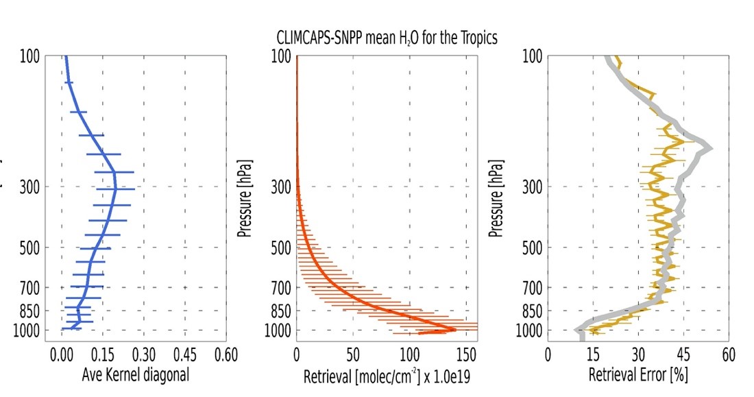
In Figure 3 and Figure 4 we take a closer look at CLIMCAPS averaging kernels, H₂O profile retrievals and their associated errors. We plot these for CLIMCAPS-SNPP on 1 April 2016. Figure 3 shows the mean profiles (with standard deviation error bars) for the Tropics (30°South to 30°North), and Figure 4 for the North Polar region (> 60°North). We used the diagonal vector of the averaging kernel matrix as representation of the maximum sensitivity at each pressure layer.

The blue line (Figure 3 and Figure 4) is the mean of the diagonal vectors in each latitudinal zone, respectively. Note how there are fewer vertical error bars on the blue line compared to the retrieval (orange line) and error (yellow line) profiles. This is because the 2-D averaging kernel matrices are written to the product file on the trapezoid pressure layers to save space. The retrieval and its error covariance matrix are, however, written out on the standard 100 pressure layers as 1-D arrays.

Figure 3: A diagnosis of CLIMCAPS-SNPP H₂O vapor retrievals in the tropics [>30°S, <30°N] on 1 April 2016. Each solid line represents the mean zonal profile with error bars defined by the standard deviation at each pressure layer. [left] CLIMCAPS H₂O vapor averaging kernel matrix diagonal vector from netCDF field ave_kern/h2o_vap_ave_kern that indicates the pressure layers at which CLIMCAPS has sensitivity to the true state of H₂O vapor in the atmosphere. [middle] CLIMCAPS H₂O vapor profile retrieval from netCDF field mol_lay/h2o_vap_mol_lay [molec/cm²]. [right] CLIMCAPS retrieval error from netCDF field mol_lay/h2o_vap_mol_lay_err [molec/cm²] represented here as percentage [mol_lay/h2o_vap_mol_lay_err]/[ mol_lay/h2o_vap_mol_lay]⁎100. CLIMCAPS uses an empirical a-priori error estimate and is represented by the thick grey line. In calculating these mean profiles, we filtered out all retrievals where mol_lay/h2o_vap_mol_lay_qc(i,j) > 1. We plot these profiles using the pressure layer array called air_pres_lay.

We calculated an empirical error covariance matrix for the CLIMCAPS H₂O vapor a-priori (Section 2.2). The a-priori error profile in Figure 3 and Figure 4 (righthand panel, grey line) is the square root of the diagonal vector from this error covariance matrix. In Section 2.2, we plot the full error covariance matrix and also explain why you see those zig-zag patterns in the retrieval error (righthand panel, yellow profile).

A comparison between the retrieval error (yellow) and a-priori error (grey) profiles can be helpful in applications and data evaluation. As discussed elsewhere the retrieval error (mol_lay/h2o_vap_mol_lay_err) does not indicate retrieval accuracy, it does not quantify how closely the retrieval resemble the true state. Instead, the CLIMCAPS retrieval error is the a-posteriori error as described by (Rodgers, 2000) for Optimal Estimation (O-E) inversion systems.

This a-posteriori error resembles the total error budget of the retrieval system and includes the measurement error, forward model error, background state error and smoothing error (Smith and Barnet, 2019). The a-posteriori error only has meaning in comparison to the a-priori error because it quantifies how much the measurements contributed to reducing uncertainty about the prior state. The amount of information extracted from the measurements depend on the inversion system (e.g., channel selection, measurement error covariance and various stabilization parameters) and is quantified by the averaging kernel.

When we re-examine Figure 3 and Figure 4 we see that the a-posteriori error profile (righthand panel, yellow) is less than the a-priori error profile (righthand panel, grey) where the averaging kernel (left-hand panel, blue) reaches a maximum.

Figure 4: Same as Figure 3 but for the north polar zone [>60°N].

The averaging kernel diagonal vectors for the North Polar zone (Figure 4) are overall smaller and with a different shape than those in the Tropics (Figure 3). This is consistent with the DOF shown in Figure 1, where information content of H₂O is a strong function of latitude. Compared to the Tropics (Figure 3), retrievals in the North Polar zone (Figure 4) are an order of magnitude drier. In the Tropics, moisture extends high into the column since the ITCZ can produce deep convection, which can transport water molecules up to the tropopause and in some cases, into the stratosphere.

1.2  MW-only H₂O retrieval

The CLIMCAPS system has a MW-only step that retrieves temperature (mw_air_temp), H₂O column density (mw_h2o_vap_mol_lay), liquid water path (mw_h2o_liq_mol_lay), and surface emissivity (surf_mw_emis) using the method developed by (Rosenkranz, 2001, 2006), a sequential optimal estimation that uses a MW-only radiative transfer model as described by (Rosenkranz, 2003; Rosenkranz and Barnet, 2006).

The liquid water path and surface emissivity retrieved variables are propagated into subsequent CLIMCAPS retrieval steps while temperature and H₂O are written to the file as MW-only retrievals for use in research. Note that there are no corresponding averaging kernels for these MW-only retrievals.

MW-only estimates of H₂O may be useful for certain applications where cloud clearing has failed due to uniform clouds or difficult surface conditions. However, the MW-only retrieval has a lower vertical resolution than the combined IR+MW CLIMCAPS retrieval, so we recommend caution when combining these in analyses.

2. Preparing CLIMCAPS H₂O retrievals for applications

2.1 Boundary layer adjustment

CLIMCAPS uses a standard 100-layer pressure grid to retrieve atmospheric variables from Earth surface to top of atmosphere. This pressure grid is required by radiative transfer models (SARTA for CLIMCAPS) to accurately calculate top of atmosphere hyperspectral IR radiances. CLIMCAPS uses the exact same pressure grid at every scene on Earth and accounts for surface pressure as a separate variable during radiative transfer calculations. CLIMCAPS V2 uses MERRA2 surface pressure as input. The retrieved profiles are, however, reported on the 100-layer grid as a means to standardize the output. It is important that you adjust the bottom layer, i.e. that pressure layer intersecting the Earth surface as identified by air_pres_lay_nsurf in the CLIMCAPS netCDF file, to accurately reflect the total number of water vapor molecules in the boundary layer. 

You should do this boundary layer adjustment if you calculate total column densities or if you are converting moisture units from layers to levels. We describe the method for doing this adjustment in detail elsewhere.

2.2 H₂O a-priori

CLIMCAPS employs MERRA2 (Gelaro et al., 2017; GMAO, 2015) as a-priori for its T(p), water vapor and ozone retrievals. CLIMCAPS converts MERRA2 T(p) profiles from their 72 pressure levels to the standard 100 retrieval layers (air_pres_lay). Additionally, CLIMCAPS interpolates MERRA2 profiles spatially and temporally to match the measurements. These interpolated MERRA2 profiles are written to the CLIMCAPS product file as fg_air_temp, fg_h2o_mol_lay and fg_o3_mol_lay.

We describe the benefits of employing MERRA2 as a-priori in Section 2.2.3 of Smith and Barnet (2019) and also explain how we derived the a-priori error covariance matrix depicted here. In short, the a-priori error (Figure 5) is presented as percentage because we derive  as the covariance of (ECMWF – MERRA2)/ECMWF. This covariance matrix of percent difference is derived from an ensemble data set of 233,135 collocated profiles from ECMWF and MERRA2 for four global days, 1 January 2015, 1 April 2015, 1 July 2015 and 1 October 2015.

Before calculating the difference between ECMWF and MERRA2, we apply a 3-point running mean on each profile individually to smooth out fine structures. Then we filter out all cases where the absolute value of the difference between ECMWF and MERRA2 is > 50% for H₂O and > 10 K for temperature.

Figure 5: Empirical a-priori error covariance matrix used in CLIMCAPS V2 H₂O retrievals as described in Smith and Barnet (2019).

We depicted the square root of the diagonal vector of the CLIMCAPS H₂O a-priori matrix (Figure 5) as the grey profile in Figure 3 and Figure 4. Why, then, does the retrieval error profile (yellow in the same figures) have a zig-zag pattern? The simple answer is that this pattern emerges as a numerical artifact caused by our data compression methods.

As described in Smith and Barnet (2020), CLIMCAPS calculates brute force Jacobians (weighting functions) on a reduced set of pressure layers as defined by overlapping trapezoid functions. We do this to speed up processing. In addition, CLIMCAPS performs its iterative minimization equation (i.e., retrieval) in orthogonal space as a set of eigenvectors to separate signal from noise. Every time the forward model, SARTA, is called, CLIMCAPS has to reconstruct the profiles from orthogonal to physical space and then convert them back onto the 100 layers (air_pres_lay). This numerical process introduces the oscillating pattern. For example, when CLIMCAPS ingests the matrix in Figure 5 as a-priori error covariance, transform it onto trapezoid layers, compress it to orthogonal space and then reconstruct and expand again according to Eq. 1, the matrix structure changes as seen in Figure 6a.  

Eq. 1          \( (\delta (H_{2}O) \delta(H_{2}O)^{T})_{a} = G \cdot \delta (H_{2}O) \delta (H_{2}O )^{T} \cdot G \)

Where \(G = F_{Lj} \cdot U_{jk} \cdot (I − \Phi ) \dot U_{kj} \cdot F_{Lj}^{−1} \), \(U_{jk} \) is the transformation matrix from \(k\) eigenvectors to \(j\) trapezoidal layers, \(F_{Lj} \) is the transformation matrix from \(j\) to \(L\) SARTA pressure layers. The indices have the following maximum value and definition: \(k \leq 6 \) eigenvectors, \( j = 22 \) trapezoid layers, and \( L = 100\) retrieval layers.

Figure 6: CLIMCAPS V2 smoothing error, measurement error and retrieval error covariance matrices as described in Smith and Barnet (2019).

The a-posteriori, or retrieval, error covariance matrix (Figure 6c) is the sum of the smoothing error (Figure 6a) and measurement error (Figure 6b) covariance matrices. The latter is calculated as:

Eq. 2          \( (\delta (H_{2}O) \delta(H_{2}O)^{T})_{o} = Z \cdot \frac{1}{\lambda} Z^T \)

Where \( \lambda \) is the a-priori matrix, \delta (H_{2}O) \delta(H_{2}O)^{T} in orthogonal (or eigenvector) space, \(k\), and \(Z\) is the amount of measurement (or measurement noise) that is believed in retrieval space (L) such that \( Z = F \cdot U_{jk} \cdot \Phi \), where \( \Phi \) is the fraction of the parameter solved for. The square root of the diagonal vector from the a-posteriori matrix (Figure 6c) is the yellow profile in Figure 3 and Figure 4.

2.3 Retrieval Evaluation

2.3.1 Radiosondes/Dropsondes

Figure 7 shows the atmospheric structure captured by dropsondes (middle) and CLIMCAPS retrievals (bottom), respectively. The middle and bottom panels are the profiles along a NOAA research flight path, which passed over Hurricane Jerry on Sept 18, 2019 in the Atlantic Ocean. The flights were timed to coincide with the satellite overpass and are all within 2 hours of the flight.

The dropsondes, unlike radiosondes, take approximately 20 minutes to reach the surface once they are released from the aircraft. They have less horizontal drift, typically around 50 km. Dropsondes can sample over 10,000 pressure levels, which is two orders of magnitude higher than the 100 retrieval layers used in CLIMCAPS.

Despite vertical and horizontal resolution differences, we see that both the dropsondes and CLIMCAPS observe the pockets of dry air. Knowledge of dry air is useful when examining Hurricanes since they are indicators of a storm’s ability to intensify or weaken. In the case of Jerry, dry air from the Saharan Air Layer (SAL) was being entrained, but Jerry still briefly intensified to a category 3 Hurricane.

Figure 7: A research flight on September 18, 2019 shows (a) along a flight path over Hurricane Jerry the relative humidity profiles from (b) dropsondes released from a Gulfstream-IV “Hurricane Hunter” aircraft and (c) CLIMCAPS-SNPP H₂O retrievals as relative humidity. The solid line in (a) represents the flight path and the numbers are used to identify the location of the dropsonde profiles in (b) and (c). The colored dots indicate the center location of the CLIMCAPS footprint and if the retrieval passed (green) or failed (red). No averaging kernel convolution has been applied to the radiosonde data. However, for a quantitative comparison, we recommend that users apply this procedure.

We recommend work by (Nalli et al., 2018a, 2018b) that describe methods for inter-comparing satellite soundings and radiosondes.

2.3.2 Averaging Kernels

Averaging kernels are helpful when evaluating and comparing satellite sounding retrievals as discussed in these publications (Iturbide-Sanchez et al., 2018; Maddy and Barnet, 2008; Smith and Barnet, 2020). We outline a method for convolving radiosondes (or model profiles) with CLIMCAPS averaging kernels to remove differences due to vertical resolution.

2.4 Units of conversion

Moisture is essential for measuring many derived atmospheric stability parameters. To facilitate these calculations, there are numerous ways to measure the water content of the atmosphere. CLIMCAPS retrieves moisture in column density with units of molec/m² (mol_lay/ h2o_vap_mol_lay). In addition, the netCDF file contains a number of derived values, including relative humidity (rel_hum), specific humidity (spec_hum) and TPW (h2o_vap_tot). We describe unit conversions for H₂O elsewhere.

3. Relevant fields in file

3.1 Retrieved variables

• mol_lay/ h2o_vap_mol_lay: CLIMCAPS retrieval of H₂O vapor layer column densities [molec/m²] on 100 pressure layers (air_pres_lay). Multiply by 1.0e-04 to convert to the more common form of [molec/cm²]. measurements.
• mw/mw_h2o_vap_mol_lay: Microwave-only retrieval of H₂O vapor layer column densities [molec/m²] on 100 pressure layers (air_pres_lay). Multiply by 1.0e-04 to convert to the more common form of [molec/cm²].

3.2 Derived variables

• rel_hum: Relative humidity [%] derived from mol_lay/ h2o_vap_mol_lay, reported on 66 pressure layers (air_pres_h2o).
• h2o_vap_tot: Total mass of water vapor content [kg/m²] derived from mol_lay/ h2o_vap_mol_lay. Also known as Total Precipitable Water, or TPW in units [mm], because 1 kg/m²= 1 mm. TPW refers to the gaseous form of water in the atmosphere, not water droplets in clouds.
• spec_hum: specific humidity [kg/kg], which is the mass fraction of H₂O in total air derived from mol_lay/ h2o_vap_mol_lay and reported on 66 pressure layers (air_pres_h2o).
• spec_hum_sat_ice: saturation specific humidity over ice and reported on 66 pressure levels (air_pres_h2o) derived from
• spec_hum_sat_liq: saturation specific humidity over liquid water and reported on 66 pressure levels (air_pres_h2o).
• mw/mw_h2o_vap_tot: Total mass of water vapor content [kg/m²] derived from mw/mw_h2o_vap_mol_lay. Also known as Total Precipitable Water, or TPW in units [mm], because 1 kg/m²= 1 mm. TPW refers to the gaseous form of water in the atmosphere, not water droplets in clouds.
• mw/mw_spec_hum: Specific humidity, the mass fraction of water vapor in total air, from the MW-only step [kg/kg] derived from mw/mw_h2o_vap_mol_lay and reported on 66 pressure layers (air_pres_h2o).

3.3 Quality metrics

• ave_kern/h2o_vap_ave_kern: H₂O vapor averaging kernel matrix for every retrieval scene.
• h2o_vap_dof: The trace of the averaging kernel matrix as a measure of the number of independent pieces of information about H₂O at a target scene. For H₂O, CLIMCAPS typically maintain a DOF below 4, which means that CLIMCAPS has sensitivity to the true state of H₂O at a target scene in three vertical layers.
• *_err: The retrieval error estimate for column density (h2o_vap_mol_lay), relative humidity (rel_hum), specific humidity (spec_hum), and column total (h2o_vap_tot). The error has the same units as the original retrieved or derived variables.
• *_qc: The quality control flag for retrieved H₂O in several units of measure: column density (h2o_vap_mol_lay), relative humidity (rel_hum), specific humidity (spec_hum), and column total (h2o_vap_tot). This is the same quality flag used in the retrieved and derived variables.

3.4 H₂O a-priori

• aux/fg_h2o_vap_mol_lay: MERRA2 a-priori for H₂O retrieval in the MW-only and MW+IR retrieval steps. These the native MERRA2 H₂O profiles converted to column densities [molec/m²] and interpolated spatially, temporally and vertically to match the CLIMCAPS retrieval footprints. This field is included in the netCDF file so that you can readily compare the retrieval with its a-priori.

4. Publications

• Dessler, A. E. and Wong, S.: Estimates of the Water Vapor Climate Feedback during El Niño–Southern Oscillation, Journal of Climate, 22(23), 6404–6412, doi:10.1175/2009JCLI3052.1, 2009.
• Dessler, A. E., Zhang, Z. and Yang, P.: Water-vapor climate feedback inferred from climate fluctuations, 2003–2008, Geophysical Research Letters, 35(20), doi:10.1029/2008GL035333, 2008.
• Gelaro, R., McCarty, W., Suárez, M. J., Todling, R., Molod, A., Takacs, L., Randles, C. A., Darmenov, A., Bosilovich, M. G., Reichle, R., Wargan, K., Coy, L., Cullather, R., Draper, C., Akella, S., Buchard, V., Conaty, A., da Silva, A. M., Gu, W., Kim, G.-K., Koster, R., Lucchesi, R., Merkova, D., Nielsen, J. E., Partyka, G., Pawson, S., Putman, W., Rienecker, M., Schubert, S. D., Sienkiewicz, M. and Zhao, B.: The Modern-Era Retrospective Analysis for Research and Applications, Version 2 (MERRA-2), Journal of Climate, 30(14), 5419–5454, doi:10.1175/JCLI-D-16-0758.1, 2017.
• Iturbide-Sanchez, F., da Silva, S. R. S., Liu, Q., Pryor, K. L., Pettey, M. E. and Nalli, N. R.: Toward the Operational Weather Forecasting Application of Atmospheric Stability Products Derived From NUCAPS CrIS/ATMS Soundings, IEEE Transactions on Geoscience and Remote Sensing, 56(8), 4522–4545, doi:10.1109/TGRS.2018.2824829, 2018.
• Maddy, E. S. and Barnet, C. D.: Vertical Resolution Estimates in Version 5 of AIRS Operational Retrievals, IEEE Transactions on Geoscience and Remote Sensing, 46(8), 2375–2384, doi:10.1109/TGRS.2008.917498, 2008.
• Nalli, N. R., Gambacorta, A., Liu, Q., Barnet, C. D., Tan, C., Iturbide-Sanchez, F., Reale, T., Sun, B., Wilson, M., Borg, L. and Morris, V. R.: Validation of Atmospheric Profile Retrievals From the SNPP NOAA-Unique Combined Atmospheric Processing System. Part 1: Temperature and Moisture, IEEE Transactions on Geoscience and Remote Sensing, 56(1), 180–190, doi:10.1109/TGRS.2017.2744558, 2018a.
• Nalli, N. R., Gambacorta, A., Liu, Q., Tan, C., Iturbide-Sanchez, F., Barnet, C. D., Joseph, E., Morris, V. R., Oyola, M. and Smith, J. W.: Validation of Atmospheric Profile Retrievals from the SNPP NOAA-Unique Combined Atmospheric Processing System. Part 2: Ozone, IEEE Transactions on Geoscience and Remote Sensing, 56(1), 598–607, doi:10.1109/TGRS.2017.2762600, 2018b.
• Rodgers, C. D.: Inverse methods for atmospheric sounding: theory and practice, World Scientific, Singapore; Hackensack, N.J., 2000.
• Rosenkranz, P. W.: Retrieval of temperature and moisture profiles from AMSU-A and AMSU-B measurements, IEEE Transactions on Geoscience and Remote Sensing, 39(11), 2429–2435, doi:10.1109/36.964979, 2001.
• Rosenkranz, P. W.: Rapid radiative transfer model for AMSU/HSB channels, IEEE Transactions on Geoscience and Remote Sensing, 41(2), 362–368, doi:10.1109/TGRS.2002.808323, 2003.
• Rosenkranz, P. W.: Cloud liquid-water profile retrieval algorithm and validation, Journal of Geophysical Research, 111(D9), doi:10.1029/2005JD005832, 2006.
• Rosenkranz, P. W. and Barnet, C. D.: Microwave radiative transfer model validation, Journal of Geophysical Research, 111(D9), doi:10.1029/2005JD006008, 2006.
• Smith, N. and Barnet, C. D.: Uncertainty Characterization and Propagation in the Community Long-Term Infrared Microwave Combined Atmospheric Product System (CLIMCAPS), Remote Sensing, 11(10), 1227, doi:10.3390/rs11101227, 2019.
• Smith, N. and Barnet, C. D.: CLIMCAPS observing capability for temperature, moisture, and trace gases from AIRS/AMSU and CrIS/ATMS, Atmos. Meas. Tech., 13, 4437–4459, https://doi.org/10.5194/amt-13-4437-2020, 2020.