News | March 30, 2010
Global distribution and increase of carbon dioxide in the mid-troposphere, 2002-2009
This visualization is a time-series made with data retrieved by the Atmospheric Infrared Sounder (AIRS) on the NASA Aqua spacecraft. For comparison, it is overlain with a graph of the seasonal variation and interannual increase of carbon dioxide measured at the Mauna Loa Observatory in Hawaii.
This visualization is a time-series of the global distribution and variation of the concentration of mid-tropospheric carbon dioxide observed by the Atmospheric Infrared Sounder (AIRS) on the NASA Aqua spacecraft. For comparison, it is overlain by a graph of the seasonal variation and interannual increase of carbon dioxide observed at the Mauna Loa, Hawaii observatory.
The AIRS data show the average concentration (parts per million) over an altitude range of 3 km to 13 km, whereas the Mauna Loa data show the concentration at an altitude of 3.4 km and its annual increase at a rate of approximately 2 parts per million (ppm) per year.
The two most notable features of this visualization are the seasonal variation of CO2 and the trend of increase in its concentration from year to year. The global map clearly shows that the CO2 in the northern hemisphere peaks in April-May and then drops to a minimum in September-October.
Although the seasonal cycle is less pronounced in the southern hemisphere it is opposite to that in the northern hemisphere. This seasonal cycle is governed by the growth cycle of plants. The northern hemisphere has the majority of the land masses, and so the amplitude of the cycle is greater in that hemisphere. The overall color of the map shifts toward the red with advancing time due to the annual increase of CO2.
Although the mid-latitude jet streams are not visible in the map, we can see their influence upon the distribution of CO2 around the globe. These rivers of air occur at an altitude of about 5 km and rapidly transport CO2 around the globe at that altitude. In the northern hemisphere, the mid-latitude jet stream squirms like a released garden hose over the period of a few days due to the continental landmasses.
In the southern hemisphere the jet stream flow is more directly West to East, and during the period from July to October the CO2 concentration is enhanced in a belt delineated by the jet stream and lofting of CO2 into the free troposphere by the high Andes is visible in this period. The zonal flow of CO2 around the globe at the latitude of South Africa, southern Australia and southern South America is readily apparent.
Eastward flow of CO2 from Indonesia and the Celebes sea can be seen in the November to February time frame.
More versions and formats
To access other formats of this visualization, click the link below. Versions of this visualization are available at 24 seconds and 48 second lengths.
AIRS CO2 Visualization at the Scientific Visualization Studio at NASA/GSFC
More CO2 from AIRS
Image Credits
Animators:
Lori Perkins (Lead), NASA/GSFC
Greg Shirah, NASA/GSFC
Scientists:
Moustafa Chahine, NASA/JPL
Tom Pagano, NASA/JPL
Edward Olsen, NASA/JPL
Luke Chen, NASA/JPL